How to calculate IRR (Internal Rate Of Return) in Excel
IRR is the acronym for Internal Rate Of Return.It is defined in the terms of NPV or Net Present Value. The IRR can be stated as the discount rate that makes the NPV of all cash flows ( both positive and negative cash flows) from a project or investment equal to zero. It's one of the most important financial tool to evaluate the desirability of a potential project or investment. A higher IRR than the company's own acceptable rate indicates the project or investment is likely to give good return in future. Whereas, the lower IRR indicates poor return on investment.
IRR can be easily calculated with our online irr calculator, which is an excellent tool to get quick result. However, for offline use, you can still prefer using the spreadsheet programs like Excel, Libreoffice Calc, OpenOffice Calc, etc. Let's find out, how to calculate IRR in Excel spreadsheet. The method for calculating IRR in other spreadsheets is almost same.
Formula for IRR in Excel
The formula or function for calculating IRR in excel considers the initial investment as the first cash flow (negative Cash flow). So the formula ( or function) for calculating IRR in Excel is :
IRR(value1,value2,... )
In the above formula the value1 would be the initial investment (Period 0 with negative cash flow) followed by cash flows from all other periods.
IRR calculation in Excel with example
Using the above mentioned formula, let's find out how to calculate IRR in an Excel Spreadsheet with a real world example. Given below is a table with cash flows data for different period. The initial investment made in a project is $5000. So, cash flow for period 0 will be -5000. Since the cash is flowing outwards for period 0, that's why it is considered as negatve cash flow. All other cash flows are given into the table. Based on these given data, we would calculate the Internal Rate of Return in Excel.
| Cash Flows | |
| Period 0 (Initial Investment) | -5000 |
| Period 1 | 1000 |
| Period 2 | -150 |
| Period 3 | 3000 |
| Period 4 | -700 |
| Period 5 | 2500 |
| Period 6 | 900 |
Step 1: Getting all values inside Excel
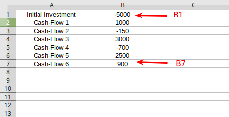
First you have to fill in the data inside the cells of Excel. You can start with any row or column but in this case we'll start with extreme left column A and column B. Let the column A should contain the cash-flow period and the column B should have it's corresponding values (either positive or negative) depending upon the data given into the example above. The initial investment or period 0 will be into the first row under colum B that's why it's cell is B1. Similarly, other values are written under column B. The cash-flow count starts with B1 cell and ends upto B7 cell as shown in the picture below.

Step 2: Appying Excel Formula inside a cell
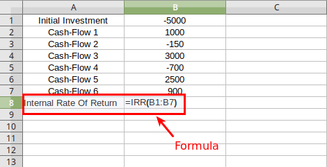
Since, the values of cash flows starts with B1 and goes upto B7 cell. Now, we have all the values ready to be applied inside the function to get the IRR result. Let's select a new cell under the last cash flow and name it as "internal rate of return". The corresponding cell B8 should have the IRR value. Based upon the above mentionded formula type "=IRR(B1:B7)". Here (B1:B7) is equivalent to (B1,B2,B3,....,B7).

Step 3: Finally, Getting the result
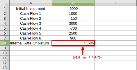
Finally, after typing the above function inside the B8 cell hit enter. This will automatically return the IRR inside the same cell (B8) in percentage. Therefore, the IRR for this example would be 7.59%

The IRR of 7.59% would be acceptable case for desirability of a project or investment. That's it, this is how you can calculate IRR inside Excel
Read More : How to calculate NPV in Excel.
Read More : How to calculate CAGR in Excel.